Information and FAQs
General Information
EDA Explorer is a site where anyone with EDA data can upload it for automatic artifact and peak detection and visualization. Settings can be customized and the results can be downloaded in CSV format. You can also use the "Label Epochs" feature to plot your raw data in 5-second epochs, which you can then label as "good" or "bad." You can then download the results to train your own classifier. See demos of all these features here.
Sara Taylor and Natasha Jaques from the MIT Media Lab's Affective Computing group designed the peak and artifact detection algorithms and created the website. The website has been improved and is maintained by Victoria Xia.
You can view the paper related to this work and/or download their scripts by going to the main page. Contact Sara and Natasha at <sataylor (at) mit.edu> and <jaquesn (at) mit.edu> with any questions, comments, or suggestions for new features. Thanks for visiting!
You can view the paper related to this work and/or download their scripts by going to the main page. Contact Sara and Natasha at <sataylor (at) mit.edu> and <jaquesn (at) mit.edu> with any questions, comments, or suggestions for new features. Thanks for visiting!
Dashboard
The dashboard is where you can see all your saved files and labeling progress in one place, as well as where you can change your account settings and invite new members to join your team.
Your dashboard shows the following types of files:
- Raw files: These are EDA data you upload in Q sensor, E4 sensor, or Shimmer sensor format. These files will be used to create the other types of files. Raw files downloaded from the dashboard are in Q sensor format.
- Peak files: These are created by going to "Find Peaks" and selecting the raw file and peak extraction settings you'd like to use. See below for more details.
- Noise files: These are created by going to "Find Noise" and selecting the raw file you'd like to use. See below for more details.
- Epoch files: These are created by going to "Label Epochs" and selecting a raw file. See below for more details.
A "peak extraction setting" is a set of preferences that can be used when you visualize peaks. See below for more details.
There are three team account settings you can change:
- Account name: Self-explanatory.
- Number of team members to label each epoch file: A positive integer indicating how many label sets you'd like for each epoch file. This number appears in the "Number of label sets" column of the "Epoch Files" table on the dashboard, so your team members can easily see which files need more labels.
- Number of skips per epoch: A positive integer indicating, when labeling epochs, how many times each person can skip a particular epoch before the epoch will not be shown again (to that person). This way, if there's an epoch you don't want to label, it won't keep re-appearing.
If you have deleted the raw file used to generate a peak/artifact file, you will not be able to automatically re-visualize that file. (The same is true if you have deleted the peak extraction setting used to generate a peak file.) Similarly, if you have deleted the raw file used to generate an epoch file, you will not be able to label it further.
Finding Peaks
The first plot shows your raw EDA data in blue, with peaks marked in green. The bottom graph shows accelerometer data, with the three colors corresponding to the three directions of movement (X is blue, Y is green, Z is red).
The minimum amplitude a potential SCR must reach in order to be counted as an SCR.
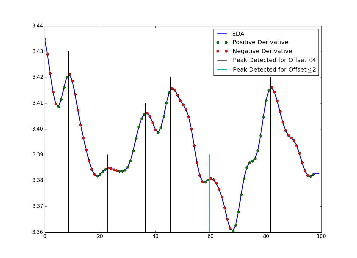
The number of seconds for which the derivative must be positive before a peak and the number of seconds for which the derivative must be negative after a peak.
The following image displays this concept visually. The blue line show the EDA signal. The red circles mark the samples that have a negative derivative and the green circles mark the samples that have a positive derivative. Assuming the signal was sampled at 8 Hz, the 5 black vertical lines show peaks that have been detected when the offset has been set to 0.5 seconds (4 samples) or lower. We can see that the there are at least 4 green circles before the detected peak and at least 4 red circles after the detected peak. Note that the peak that is marked with a vertical cyan line is not detected as a peak when the offset is set to greater than 0.25 seconds (2 samples) because it only has 2 samples with positive derivatives before the peak. Also, notice that the last peak marked (near sample 80) would also be detected for an offset up to 1.75 seconds (14 samples) because of the many increasing samples before the peak and the many decreasing samples after the peak.
The following image displays this concept visually. The blue line show the EDA signal. The red circles mark the samples that have a negative derivative and the green circles mark the samples that have a positive derivative. Assuming the signal was sampled at 8 Hz, the 5 black vertical lines show peaks that have been detected when the offset has been set to 0.5 seconds (4 samples) or lower. We can see that the there are at least 4 green circles before the detected peak and at least 4 red circles after the detected peak. Note that the peak that is marked with a vertical cyan line is not detected as a peak when the offset is set to greater than 0.25 seconds (2 samples) because it only has 2 samples with positive derivatives before the peak. Also, notice that the last peak marked (near sample 80) would also be detected for an offset up to 1.75 seconds (14 samples) because of the many increasing samples before the peak and the many decreasing samples after the peak.
We use a Butterworth lowpass filter, so the filter frequency is the cutoff frequency (in Hz) of this filter.
We use a Butterworth lowpass filter, so the filter order is the number of poles/zeros in the filter. The higher the order the steeper the cutoff on the filter; however, higher orders take longer to compute.
The maximum number of seconds before the apex of a peak that is the "start" of the peak.
The maximum number of seconds after the apex of a peak that is the "rec.t/2" of the peak, 50% of amp
This button will add a new row into the "Peak Extraction Settings" table on your dashboard. The next time you visualize peaks, you will have the option to select this entire set of settings, so you don't have to re-enter the numbers each time.
Pressing this button will add a new row into the "Peak Files" table on your dashboard, from which you can download the created file. The file contains computed features for each of the peaks displayed in the current visualization. See below for details about these features.
Note that pressing this button will automatically save the settings used as a new "peak extraction setting" and add it to your dashboard, if it hasn't been saved already.
Note that pressing this button will automatically save the settings used as a new "peak extraction setting" and add it to your dashboard, if it hasn't been saved already.
Finding Noise
The first plot shows your EDA data. Noise is shaded red, and questionable regions are shaded gray. (Note that gray regions will only appear if the "Multiclass" classifier setting is selected.) The second plot shows accelerometer data, with the three colors corresponding to the three directions of movement (X is blue, Y is green, Z is red).
The binary classifier classifies data into one of two categories: clean or noise. The multiclass classifier classifies data into one of three categorires: clean, noise, or unsure/questionable.
Pressing this button will add a new row into the "Noise Files" table on your dashboard, from which you can download the file. The first column of this file contains time-stamps that break your raw data into 5-second epochs. The second column contains either a -1, 1, or 0 in each row, representing whether the corresponding epoch is a noise, is clean, or is questionable.
Labeling Epochs
You will see one figure at a time with 4 plots in order to help you decide how to label the section of EDA signal shown. Each figure represents a 5-second epoch of the raw file you chose to label.
The X-axis is in seconds since the start of your EDA data. Note that the bottom three plots share a common X-axis, while the top plot has a smaller one. The shaded area of the bottom three plots corresponds to the X-axis range of the top one.
On the EDA plots, the Y-axis is in µSiemens and will span at least 0.5 µSiemens
On the Acceleration plot, the Y-axis is in g’s and will span at least 1.0 g's.
On the Temperature plot, the Y-axis is in °C and will span at least 1°C.
On the Acceleration plot, the Y-axis is in g’s and will span at least 1.0 g's.
On the Temperature plot, the Y-axis is in °C and will span at least 1°C.
Pressing the arrow skips this epoch for now. Skipped epochs will be displayed the next time you begin labeling the same file again, unless you have skipped the epoch the maximum number of times allowed (See "Why do epochs I didn't label sometimes disappear?" below.).
Each row of this file corresponds to a 5-second epoch of the raw file used to create it. The "epoch number" and "epoch start time" columns are self-explanatory. The additional columns correspond to each member of your team who has started labeling these epochs. A label of 1 is generated using the check mark, a label of 2 is generated using the "x", and 0 means no label has been assigned.
There is an account setting that specifies the maximum number of times an epoch can be skipped before it disappears, so you don't have to keep skipping epochs you don't want to label. You can change this setting by going to "change account preferences" on your dashboard.
Peak Files: Computed Features
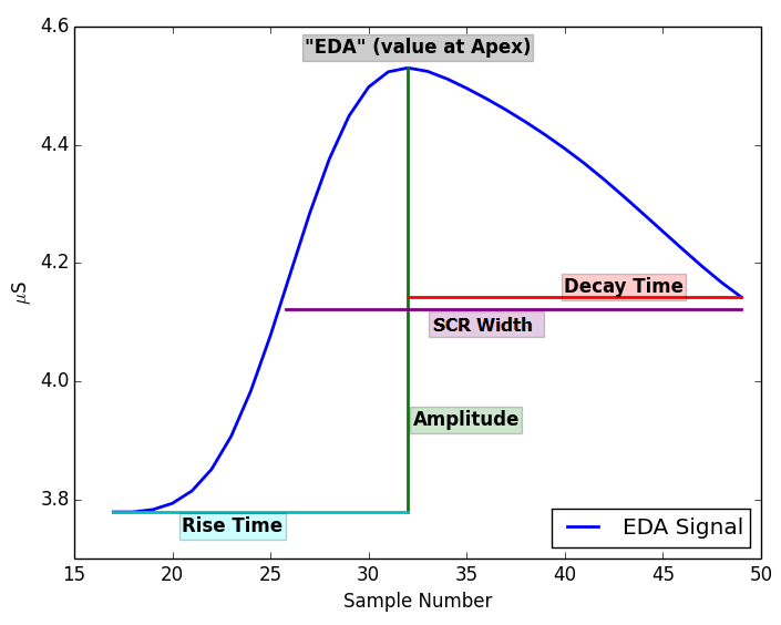
The timestamp of the apex of the peak. This is the index of the feature file (the first column).
The EDA amplitude at the apex, in µSiemens.
The time, in seconds, it takes for the SCR to rise from the start of the SCR to the apex.
The start of the SCR is computed by going backwards from the apex of the peak to point where derivative is less than 1% of its maximum value.
The start of the SCR is computed by going backwards from the apex of the peak to point where derivative is less than 1% of its maximum value.
Maximum derivative of SCR, in µSiemens per second.
Amplitude of peak; that is [amp = (EDA at apex) - (EDA at start of the SCR)], in µSiemens.
The time, in seconds, that it takes for the SCR to decay to 50% of its amplitude. Note that this is blank if an SCR doesn’t decay to 50% before another peak starts or before the maximum decay time is reached.
The time in seconds between the 50% of the amplitude on the incline side of the peak to 50% of the amplitude on the decline side of the SCR.
Note that this is blank if a Decay_time wasn’t computed.
Note that this is blank if a Decay_time wasn’t computed.
Area under the Curve; approximated by multiplying the Amplitude by the SCR_width. Note that this is blank if a Decay_time wasn’t computed.